Great variety of wideband antenna solutions
COJOT is a well-respected and long established Finnish company, designing and developing omnidirectional VHF/UHF/SHF wideband antennas and accessories for mobile tactical communication, electronic warfare and spectrum monitoring applications.
Browse our products